How To Simulate Patch Attacks
Introduction
This notebook provides a beginner friendly introduction to using adversarial patches for object detection as part of Test & Evaluation with the VisDrone dataset. We first run the attack with the default parameters, and then go through the parameters to understand their effect on the resulting patch. In each case, we visualize the resulting patch and the detector’s output under test. Computing the performance under such patch attacks is a crucial step in T&E.
❗Patches can be effective simply by covering the target object. This should be taken into account when evaluating❗
Intended Audience: All T&E Users
Requirements: Basic Python and Torchvision / ML Skills
Notebook Runtime: Full run of the notebook: <4 minutes
Reading time: ~10 Minutes
Order of Completion: Order in the guide.
Before you begin, you will want to make sure that you download the how-to guide’s companion Jupyter notebook. This notebook allows you to follow along in your own environment and interact with the code as you learn. The code snippets are also included in the documentation, but the notebook is provided for ease of use and to enable you to try things on your own.
Note
The How to Craft a Patch for Object Detection Notebook can be downloaded via the HEART public GitHub.
Contents
Imports and set-up
Load data and model
Initialize patch attack
Patch shape
Patch position
Patch Type
Conclusion
Next steps
Learning Objectives
how to apply a patch attack using JATIC
Which parameters a patch attack uses
How changing these parameters affects the resulting patch
1. Imports and Set-up
We import all necessary libraries for this tutorial. In this order, we first import general libraries such as numpy, then load relevant methods from ART. We then load the corresponding HEART functionality and specific torch functions to support the model. Lastly, we use a command to plot within the notebook.
# general imports
import numpy as np
from functools import partial
from pprint import pprint
import cv2
import matplotlib.pyplot as plt
from typing import Tuple, Dict, Any
from copy import deepcopy

# imports from ART
from art.attacks.evasion import AdversarialPatchPyTorch

# imports from HEART
from heart_library.estimators.object_detection import JaticPyTorchObjectDetector
from heart_library.attacks.attack import JaticAttack
from heart_library.metrics import AccuracyPerturbationMetric
from heart_library.metrics import HeartMAPMetric, HeartAccuracyMetric

# dataset imports
from datasets import load_dataset
from datasets import Dataset

# torch imports
import torch
from torchvision.transforms import transforms

# MAITE imports
from maite.protocols.object_detection import TargetBatchType
from maite.workflows import evaluate
from maite.protocols.object_detection import Dataset as od_dataset
from maite.protocols.image_classification import Augmentation
from maite.utils.validation import check_type

plt.style.use('ggplot')
%matplotlib inline
Before loading data and model, we define a couple of methods that we will use later on on the drone data. These encompass getting predictions with a confidence threshold, plotting input images with the predicted bounding boxes, and a special wrapper for image data.
# given a confidence threshold, determine which of the mdoel's predictions are relevent
def extract_predictions(predictions_, conf_thresh):
    # Get the predicted class
    predictions_class = [visdrone_labels[i] for i in list(predictions_.labels)]
    #  print("\npredicted classes:", predictions_class)
    if len(predictions_class) < 1:
        return [], [], []
    # Get the predicted bounding boxes
    predictions_boxes = [[(i[0], i[1]), (i[2], i[3])] for i in list(predictions_.boxes)]

    # Get the predicted prediction score
    predictions_score = list(predictions_.scores)
    # print("predicted score:", predictions_score)

    # Get a list of index with score greater than threshold
    threshold = conf_thresh
    predictions_t = [predictions_score.index(x) for x in predictions_score if x > threshold]
    if len(predictions_t) > 0:
        predictions_t = predictions_t  # [-1] #indices where score over threshold
    else:
        # no predictions esxceeding threshold
        return [], [], []
    # predictions in score order
    predictions_boxes = [predictions_boxes[i] for i in predictions_t]
    predictions_class = [predictions_class[i] for i in predictions_t]
    predictions_scores = [predictions_score[i] for i in predictions_t]
    return predictions_class, predictions_boxes, predictions_scores

#plot an image with objects with the predicted bounding boxes on top
def plot_image_with_boxes(img, boxes, pred_cls, title):
    img = (img*255).astype(np.uint8)
    text_size = 1.5
    text_th = 2
    rect_th = 2

    for i in range(len(boxes)):
        cv2.rectangle(img, (int(boxes[i][0][0]), int(boxes[i][0][1])), (int(boxes[i][1][0]), int(boxes[i][1][1])),
                      color=(0, 255, 0), thickness=rect_th)
        # Write the prediction class
        cv2.putText(img, pred_cls[i], (int(boxes[i][0][0]), int(boxes[i][0][1])), cv2.FONT_HERSHEY_SIMPLEX, text_size,
                    (0, 255, 0), thickness=text_th)

    plt.figure()
    plt.axis("off")
    plt.title(title)
    plt.imshow(img, interpolation="nearest")
    # plt.show()

#wrapper for image datasets
class ImageDataset:

    metadata = {"id": "example"}

    def __init__(self, images, groundtruth, threshold=0.8):
        self.images = images
        self.groundtruth = groundtruth
        self.threshold = threshold

    def __len__(self)->int:
        return len(self.images)

    def __getitem__(self, ind: int) -> Tuple[np.ndarray, np.ndarray, Dict[str, Any]]:
        image = np.asarray(self.images[ind]["image"]).astype(np.float32)

        filtered_detection = self.groundtruth[ind]
        filtered_detection.boxes = filtered_detection.boxes[filtered_detection.scores>self.threshold]
        filtered_detection.labels = filtered_detection.labels[filtered_detection.scores>self.threshold]
        filtered_detection.scores = filtered_detection.scores[filtered_detection.scores>self.threshold]

        return (image, filtered_detection, None)

# specific dataset class to craft a targeted adversarial patch
class TargetedImageDataset:

    metadata = {"id": "example"}

    def __init__(self, images, groundtruth, target_label, threshold=0.5):
        self.images = images
        self.groundtruth = groundtruth
        self.target_label = target_label
        self.threshold = threshold

    def __len__(self)->int:
        return len(self.data)

    def __getitem__(self, ind: int) -> Tuple[np.ndarray, np.ndarray, Dict[str, Any]]:
        image = self.images.__getitem__(ind)["image"]
        targeted_detection = self.groundtruth[ind]
        targeted_detection.boxes = targeted_detection.boxes[targeted_detection.scores>self.threshold]
        targeted_detection.scores = np.asarray([1.0]*len(targeted_detection.boxes))
        targeted_detection.labels = [self.target_label]*len(targeted_detection.boxes)
        return (image, targeted_detection, {})
2. Load Data and Model
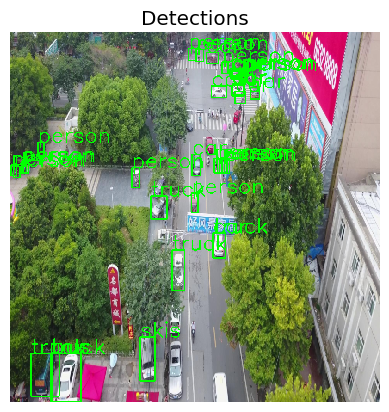
We load the data, importing only a small part (5 samples) to save compute for this small demonstration. We then define the model and wrap it as a JATIC PyTorch classifier and test its output on our samples.
visdrone_labels = [
    'N/A', 'person', 'bicycle', 'car', 'motorcycle', 'airplane', 'bus',
    'train', 'truck', 'boat', 'traffic light', 'fire hydrant', 'N/A',
    'stop sign', 'parking meter', 'bench', 'bird', 'cat', 'dog', 'horse',
    'sheep', 'cow', 'elephant', 'bear', 'zebra', 'giraffe', 'N/A', 'backpack',
    'umbrella', 'N/A', 'N/A', 'handbag', 'tie', 'suitcase', 'frisbee', 'skis',
    'snowboard', 'sports ball', 'kite', 'baseball bat', 'baseball glove',
    'skateboard', 'surfboard', 'tennis racket', 'bottle', 'N/A', 'wine glass',
    'cup', 'fork', 'knife', 'spoon', 'bowl', 'banana', 'apple', 'sandwich',
    'orange', 'broccoli', 'carrot', 'hot dog', 'pizza', 'donut', 'cake',
    'chair', 'couch', 'potted plant', 'bed', 'N/A', 'dining table', 'N/A',
    'N/A', 'toilet', 'N/A', 'tv', 'laptop', 'mouse', 'remote', 'keyboard',
    'cell phone', 'microwave', 'oven', 'toaster', 'sink', 'refrigerator', 'N/A',
    'book', 'clock', 'vase', 'scissors', 'teddy bear', 'hair drier',
    'toothbrush'
]

NUM_SAMPLES = 5

data = load_dataset("Voxel51/VisDrone2019-DET", split="train", streaming=True)
sample_data = data.take(NUM_SAMPLES)

def gen_from_iterable_dataset(iterable_ds):
    yield from iterable_ds

sample_data = Dataset.from_generator(partial(gen_from_iterable_dataset, sample_data), features=sample_data.features)

IMAGE_H, IMAGE_W = 800, 800

preprocess = transforms.Compose([
    transforms.Resize((IMAGE_H, IMAGE_W)),
    transforms.ToTensor()
])

sample_data = sample_data.map(lambda x: {"image": preprocess(x["image"]), "label": None})
MEAN = [0.485, 0.456, 0.406]
STD = [0.229, 0.224, 0.225]
preprocessing=(MEAN, STD)

detector = JaticPyTorchObjectDetector(model_type="detr_resnet50",
                                      device_type='cpu',
                                    input_shape=(3, 800, 800),
                                    clip_values=(0, 1),
                                    attack_losses=("loss_ce",),
                                    preprocessing=(MEAN, STD))

detections = detector(sample_data)

# plot the input images with the corresponding classification output
for i in range(2): # to plot all: range(len(sample_data))):
    preds_orig = extract_predictions(detections[i], 0.5)
    img = np.asarray(sample_data.__getitem__(i)['image']).transpose(1,2,0)
    plot_image_with_boxes(img=img.copy(), boxes=preds_orig[1], pred_cls=preds_orig[0], title="Detections")

3. Initialize Patch Attack
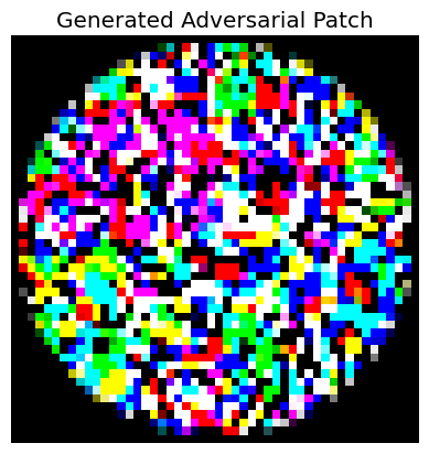
We will now initialize the patch attack and apply it before investigating individual parameters.
##### prepare dataset
targeted_data = TargetedImageDataset(sample_data, deepcopy(detections), NUM_SAMPLES)

assert isinstance(targeted_data, od_dataset)

targeted_data = torch.utils.data.Subset(targeted_data, list(range(1)))

##### initialize patch attack parameters
rotation_max=0.0
scale_min=0.5
scale_max=1.0
distortion_scale_max=0.0
learning_rate=0.9
max_iter=50
batch_size=16
patch_shape=(3, 50, 50)
patch_location=(20,20)
patch_type="circle"
optimizer="Adam"

patchAttack = JaticAttack(
    AdversarialPatchPyTorch(detector, rotation_max=rotation_max,
                      scale_min=scale_min, scale_max=scale_max, optimizer=optimizer, distortion_scale_max=distortion_scale_max,
                      learning_rate=learning_rate, max_iter=max_iter, batch_size=batch_size, patch_location=patch_location,
                      patch_shape=patch_shape, patch_type=patch_type, verbose=True, targeted=True)
    )

#Generate adversarial images
px_adv, y, metadata = patchAttack(data=targeted_data)

patch = metadata[0]["patch"]
patch_mask = metadata[0]["mask"]

#plot patch
plt.axis("off")
plt.imshow(((patch) * patch_mask).transpose(1,2,0))
_ = plt.title('Generated Adversarial Patch')
plt.show()
print('-------------')
adv_detections = detector(px_adv)
for i in range(1): #to see all, use range(len(adv_detections)):
    preds_orig = extract_predictions(adv_detections[i], 0.5)
    plot_image_with_boxes(img=px_adv[i].transpose(1,2,0).copy(),
                          boxes=preds_orig[1], pred_cls=preds_orig[0], title="Detections")
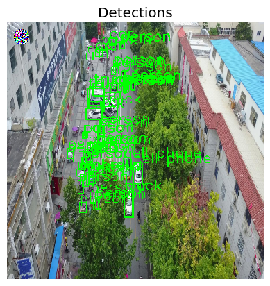
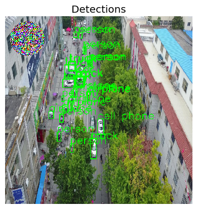
We see a small patch in the upper, left corner of the image and some differences in bounding boxes comapred to previously.
4. Patch Shape
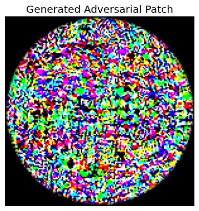
To understand the different parameters, we will now investigate each of them. Rotation, scale, and distortion determine how much the patch is reshaped during training. This can be considered data augmentation that avoids overfitting the patch. Furthermore, the learning rate, max_iter, batch-size and optimizer influence the optimization procedure. We will thus in the following investigate the remaining parameters, starting with the patch shape. This parameter denotes the size of the patch used for crafting. We increase the size, but decide to only use two instead of three color channels.
Todo: Feel free to explore the parameters by yourself and to observe the change in patch position and shape before proceeding.
##### initialize patch attack parameters
patch_shape=(3, 150, 150)
patch_location=(20,20)
patch_type="circle"

patchAttack = JaticAttack(
    AdversarialPatchPyTorch(detector, rotation_max=rotation_max,
                      scale_min=scale_min, scale_max=scale_max, optimizer=optimizer, distortion_scale_max=distortion_scale_max,
                      learning_rate=learning_rate, max_iter=max_iter, batch_size=batch_size, patch_location=patch_location,
                      patch_shape=patch_shape, patch_type=patch_type, verbose=True, targeted=True)
    )

#Generate adversarial images
px_adv, y, metadata = patchAttack(data=targeted_data)

patch = metadata[0]["patch"]
patch_mask = metadata[0]["mask"]

#plot patch
plt.axis("off")
plt.imshow(((patch) * patch_mask).transpose(1,2,0))
_ = plt.title('Generated Adversarial Patch')
plt.show()
print('-------------')
adv_detections = detector(px_adv)
for i in range(1): #to see all, use range(len(adv_detections)):
    preds_orig = extract_predictions(adv_detections[i], 0.5)
    plot_image_with_boxes(img=px_adv[i].transpose(1,2,0).copy(),
                          boxes=preds_orig[1], pred_cls=preds_orig[0], title="Detections")
As visible, the patch is now much larger, as expected when increasing the patch size. Next, we are going to alter the position of the patch.
5. Patch Position
The position denotes the offset from the upper left corner, where the patch currently appears. The image is 800 x 800, so we will shift the patch to the middle of the image, keeping the larger size set previously.
##### initialize patch attack parameters
patch_shape=(3, 150, 150)
patch_location=(300,300)
patch_type="circle"

patchAttack = JaticAttack(
    AdversarialPatchPyTorch(detector, rotation_max=rotation_max,
                      scale_min=scale_min, scale_max=scale_max, optimizer=optimizer, distortion_scale_max=distortion_scale_max,
                      learning_rate=learning_rate, max_iter=max_iter, batch_size=batch_size, patch_location=patch_location,
                      patch_shape=patch_shape, patch_type=patch_type, verbose=True, targeted=True)
    )

#Generate adversarial images
px_adv, y, metadata = patchAttack(data=targeted_data)

patch = metadata[0]["patch"]
patch_mask = metadata[0]["mask"]

#plot patch
plt.axis("off")
plt.imshow(((patch) * patch_mask).transpose(1,2,0))
_ = plt.title('Generated Adversarial Patch')
plt.show()
print('-------------')

 adv_detections = detector(px_adv)
for i in range(1): #to see all, use range(len(adv_detections)):
    preds_orig = extract_predictions(adv_detections[i], 0.5)
    plot_image_with_boxes(img=px_adv[i].transpose(1,2,0).copy(),
                          boxes=preds_orig[1], pred_cls=preds_orig[0], title="Detections")

We see that as expected, the patch is now further in the middle of the image.
❗When evaluating this patch, we have to take into account that it covers some of the objects - e.g., these will dissapear from the evaluation regardless whether the patch is effective or not ❗
6. Patch Type
So far, we have only considered round patches. In theory, a patch can have any form, but ART supports primarily round and squared patches. To conclude this notebook, we thus change the patch size to square.
##### initialize patch attack parameters
patch_shape=(3, 150, 150)
patch_location=(300,300)
patch_type="square"

patchAttack = JaticAttack(
    AdversarialPatchPyTorch(detector, rotation_max=rotation_max,
                      scale_min=scale_min, scale_max=scale_max, optimizer=optimizer, distortion_scale_max=distortion_scale_max,
                      learning_rate=learning_rate, max_iter=max_iter, batch_size=batch_size, patch_location=patch_location,
                      patch_shape=patch_shape, patch_type=patch_type, verbose=True, targeted=True)
    )

#Generate adversarial images
px_adv, y, metadata = patchAttack(data=targeted_data)

patch = metadata[0]["patch"]
patch_mask = metadata[0]["mask"]

#plot patch
plt.axis("off")
plt.imshow(((patch) * patch_mask).transpose(1,2,0))
_ = plt.title('Generated Adversarial Patch')
plt.show()
print('-------------')

adv_detections = detector(px_adv)
for i in range(1): #to see all, use range(len(adv_detections)):
    preds_orig = extract_predictions(adv_detections[i], 0.5)
    plot_image_with_boxes(img=px_adv[i].transpose(1,2,0).copy(),
                          boxes=preds_orig[1], pred_cls=preds_orig[0], title="Detections")

As expected, the resulting patch is now a square.
7. Conclusion
The adversarial patch attack learns a patch that malicously affects object detection output. Through hyperparameter tuning, both the learning process but also position, size, and shape of the patch can be altered. Special care has to be taken when it comes to the misclassification of specific objects, which can potentially be hidden behind the patch.
8. Next Steps
Check out other How-to Guides focusing on: