How to Replace Datasets in Model Evaluation

Introduction

This notebook provides a beginner friendly introduction to using different datasets in the context of JATIC and MAITE. So far, we have relied on ART to load the CIFAR10 dataset. In this notebook, we will show how to load two different datasets (MNIST and hugginface CIFAR) and how to use them within JATIC.

Intended Audience: All T&E Users

Requirements: Basic Python and Torchvision / ML Skills

Notebook Runtime: Full run of the notebook: <1 minute

Reading time: ~10 Minutes

Order of Completion: 1., then any.

Before you begin, you will want to make sure that you download the how-to guide’s companion Jupyter notebook. This notebook allows you to follow along in your own environment and interact with the code as you learn. The code snippets are also included in the documentation, but the notebook is provided for ease of use and to enable you to try things on your own.

Note

The How to Replace Datasets in Model Evaluation Companion Notebook can be downloaded via the HEART public GitHub.

Contents

1. Imports

2. Load Satellite classification data

3. Load CIFAR10 model and data from ART

4. Load CIFAR10 from Huggingface

5. Load CIFAR10 from Pytorch

6. Load Single channel dataset from Huggingface (MNIST)

7. Conclusion

8. Next Steps

Learning Objectives

• How to load the standard dataset used in the other notebooks (2.)

• Datasets can be imported from many different libraries (3.,4.,5.)

• How to load single channel (black-and-white) image data (6.)

1. Imports

We import all necessary libraries for this tutorial. In this order, we first import general libraries such as numpy, then load relevant methods from ART. We then load the corresponding HEART functionality and specific torch functions to support the model. Lastly, we use a command to plot within the notebook.

import numpy as np
import os
import requests
import matplotlib.pyplot as plt

from art.utils import load_dataset 

from heart_library.estimators.classification.pytorch import JaticPyTorchClassifier
from heart_library.metrics import AccuracyPerturbationMetric

from datasets import load_dataset as load_dataset_hf

import torch
import torchvision
from torchvision import transforms
from torchvision.models import resnet18, ResNet18_Weights

%matplotlib inline

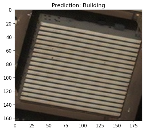
2. Load Satellite Classification Data

This way of loading a saetilte dataset is used in all other how-to’s.

 classes = {
    0:'Building',
    1:'Construction Site',
    2:'Engineering Vehicle',
    3:'Fishing Vessel',
    4:'Oil Tanker',
    5:'Vehicle Lot'
}

data = load_dataset_hf("CDAO/xview-subset-classification", split="test[0:12]")
idx = 3
plt.title(f"Prediction: {classes[data[idx]['label']]}")
plt.imshow(data[idx]['image'])

model = torchvision.models.resnet18(False)
num_ftrs = model.fc.in_features 
model.fc = torch.nn.Linear(num_ftrs, len(classes.keys())) 
model.load_state_dict(torch.load('../../../utils/resources/models/xview_model.pt'))
_ = model.eval()

Resolving data files:   0%|          | 0/31 [00:00<?, ?it/s]

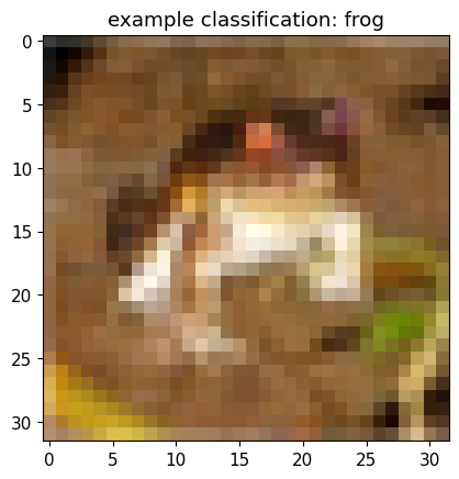
3. Load Data Using ART

(x_train, y_train), (x_test, y_test), min_, max_ = load_dataset('cifar10')
#determine number of used samples
i = 100
#reformat data to fit model
x_train = x_train[:100, :].transpose(0, 3, 1, 2).astype('float32')*255
x_test = x_test[:100, :].transpose(0, 3, 1, 2).astype('float32')*255
y_train = y_train[:100, :].astype('float32')
y_test = y_test[:100, :].astype('float32')

labels = ['airplane', 'automobile', 'bird', 'cat', 'deer', 'dog', 'frog', 'horse', 'ship', 'truck']

path = '../../../'

#model class
class Model(torch.nn.Module):
        """
        Create model for pytorch.
        Here the model does not use maxpooling. Needed for certification tests.
        """

        def __init__(self):
            super(Model, self).__init__()

            self.conv = torch.nn.Conv2d(
                in_channels=3, out_channels=16, kernel_size=(4, 4), dilation=(1, 1), padding=(0, 0), stride=(3, 3)
            )

            self.fullyconnected = torch.nn.Linear(in_features=1600, out_features=10)

            self.relu = torch.nn.ReLU()

            w_conv2d = np.load(
                os.path.join(
                    os.path.dirname(path),
                    "utils/resources/models",
                    "W_CONV2D_NO_MPOOL_CIFAR10.npy",
                )
            )
            b_conv2d = np.load(
                os.path.join(
                    os.path.dirname(path),
                    "utils/resources/models",
                    "B_CONV2D_NO_MPOOL_CIFAR10.npy",
                )
            )
            w_dense = np.load(
                os.path.join(
                    os.path.dirname(path),
                    "utils/resources/models",
                    "W_DENSE_NO_MPOOL_CIFAR10.npy",
                )
            )
            b_dense = np.load(
                os.path.join(
                    os.path.dirname(path),
                    "utils/resources/models",
                    "B_DENSE_NO_MPOOL_CIFAR10.npy",
                )
            )

            self.conv.weight = torch.nn.Parameter(torch.Tensor(w_conv2d))
            self.conv.bias = torch.nn.Parameter(torch.Tensor(b_conv2d))
            self.fullyconnected.weight = torch.nn.Parameter(torch.Tensor(w_dense))
            self.fullyconnected.bias = torch.nn.Parameter(torch.Tensor(b_dense))

        def forward(self, x):
            """
            Forward function to evaluate the model
            :param x: Input to the model
            :return: Prediction of the model
            """
            x = self.conv(x)
            x = self.relu(x)
            x = x.reshape(-1, 1600)
            x = self.fullyconnected(x)
            x = torch.nn.functional.softmax(x, dim=1)
            return x

# Define the network
model = Model()

# Define a loss function and optimizer
loss_fn = torch.nn.CrossEntropyLoss(reduction="sum")
optimizer = torch.optim.Adam(model.parameters(), lr=0.01)

# Get classifier
jptc = JaticPyTorchClassifier(
    model=model, loss=loss_fn, optimizer=optimizer, input_shape=(3, 32, 32), nb_classes=10, clip_values=(0, 255),
    preprocessing=(0.0, 255)
    
)
plt.imshow(x_train[0].transpose(1,2,0).astype(np.uint8))

pred_batch = jptc(x_train[[0]])
_ = plt.title(f'example classification: {labels[np.argmax(np.stack(pred_batch))]}')

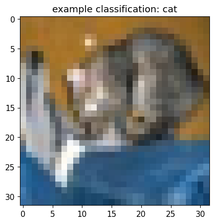
4. Load CIFAR from Huggingface

Alternative way how to load data, which is not based on ART, is to load them from huggingface. Consider that this methods has the same name as the art method, but was here renamed to avoid confusion.

#load the first ten samples of dataset
data = load_dataset_hf("cifar10", split="test[0:10]")

#output performance of previous model on data
pred_batch = jptc(data)
predictions = np.argmax(np.stack(pred_batch), axis=1)
for i, pred in enumerate(predictions[:2]):
    plt.imshow(np.asarray(data.__getitem__(i)['img']))
    plt.title(f'example classification: {labels[pred]}')
    plt.show()

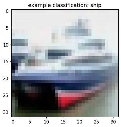
5. Loading a Dataset from Torchvision

Load CIFAR once more, this time using torchvision.

data = torchvision.datasets.CIFAR10("../data", train=False, download=True)
data = torch.utils.data.Subset(data, list(range(10)))

pred_batch = jptc(data)
predictions = np.argmax(np.stack(pred_batch), axis=1)
for i, pred in enumerate(predictions[:2]):
    plt.imshow(np.asarray(data.__getitem__(i)[0]))
    plt.title(f'example classification: {labels[pred]}')
    plt.show()

Downloading https://www.cs.toronto.edu/~kriz/cifar-10-python.tar.gz to ../data/cifar-10-python.tar.gz

100%|███████████████████████████████████████████████████████████| 170498071/170498071 [00:34<00:00, 4906438.63it/s]

Extracting ../data/cifar-10-python.tar.gz to ../data

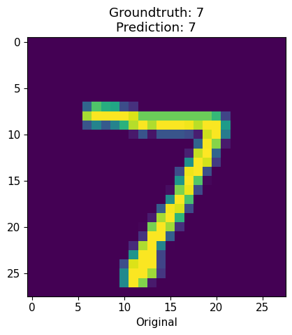
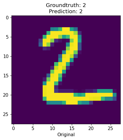
6. Single Channel Dataset from Huggingface

Lastly, we will use the huggingface model once more, but this time load a dataset with a single channel (e.g., black and white).

#simply replace name to load other dataset
data = load_dataset_hf("mnist", split="test[0:10]")
labels = list(range(10))

preprocess = transforms.Compose([
    transforms.Resize(28),
    transforms.ToTensor()
])

data = data.map(lambda x: {"image": preprocess(x["image"]), "label": x["label"]})
to_image = lambda x: transforms.ToPILImage()(torch.Tensor(x))

#load a different classifier with high performance on this task
jptc = JaticPyTorchClassifier(
    model='fxmarty/resnet-tiny-mnist', loss=loss_fn, optimizer=optimizer, input_shape=(1, 28, 28),
    nb_classes=10, clip_values=(0, 1), provider="huggingface", preprocessing=([0.45], [0.22]),
)

preds = np.stack(jptc(data))

for i in range(2):
    f, ax = plt.subplots(1,1)
    norm_orig_img = np.asarray(data.__getitem__(i)["image"]).astype(np.float32)

    ax.set_title(f'Groundtruth: {labels[data.__getitem__(i)["label"]]}\nPrediction: {labels[np.argmax(preds[i])]}')
    ax.imshow(norm_orig_img.transpose(1,2,0))
    ax.set_xlabel('Original')

model.safetensors:   0%|          | 0.00/749k [00:00<?, ?B/s]

7. Conclusion

We have seen how to load different datasets and feed them into the JATIC classifier model. With this tutorial, it should be possible to replace datasets in other how-to’s or to load a custom dataset.

8. Next Steps

Take a refresher on our previous how-to guides:

• How to Simulate White-box Attacks for Image Classification

• How to Simulate Black-box Attacks for Image Classification

• How to Simulate AutoAttack for Image Classification

• How to Create Defenses for Image Classification